TA Session 4 July: More Pandas, Parquet processing, Forecast.ETS, Database Processing and Week 4 GA#

Duration: 1h 48m

Here’s the FAQ-style transcription of the TDS live tutorial:

Q1: What is the agenda for this session?

A1: Today’s session will cover topics from week 4, go through the graded assignment, and troubleshoot any issues you encountered.

Q2: What are the tools and topics covered in Week 4?

A2: Week 4 covers using Excel for regression and forecasting, as well as Python for data analysis (reading Parquet files, data frames, pivot tables). The core idea is to be familiar with Pandas and NumPy for data manipulation in tools like Google Colab or Jupyter Notebooks, which are essential for tasks like scraping and analyzing data.

Q3: I had trouble with the last two database-related questions in the graded assignment. Can you go over them? Also, can you explain question number 7?

A3: Yes, we will definitely cover those questions.

Q4: Can you walk us through the solution for the graded assignment, starting from importing data and changing the time format?

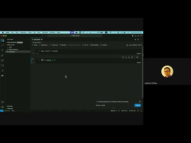
A4: Yes, I can walk you through it. I’ll start by setting up a virtual environment and then open the Parquet file using Pandas in VS Code/Colab. If you’re following along, make sure your environment is ready.

You’ll notice an error when trying to read the Parquet file because the pyarrow dependency is missing. We’ll install pyarrow first. I’ll also install numpy as it’s a great companion library to Pandas.

Once the data is loaded, the first task is to convert the “scheduled departure time” column from a decimal (float) to a more readable format. While you could use a datetime format (which I’ve covered before), I’ll show you a simpler method for this specific case. We can extract the hour by converting the float to an integer.

To convert to minutes, we’ll use a simple mathematical transformation: subtract the integer part (hours) from the original float value and then multiply by 60 to get the minutes.

For filtering, you’ll often encounter null values. It’s good practice to identify them using df.isna().any(axis=1). For this specific assignment, the solution requires treating these null values as zeros, but I want to emphasize that this is a specific case. Only do this if you are absolutely certain it’s the correct approach for your data and domain knowledge, as changing nulls to zeros can otherwise skew your analysis.

Q5: Why are we treating null values as zeros in this assignment?

A5: For this dataset, if a flight’s departure time is recorded, we can safely assume it also landed, even if the arrival time isn’t explicitly stated. In this context, a null arrival time implies it arrived on time (zero delay), making it a safe assumption to convert nulls to zeros. This specific decision is critical for obtaining the correct answers for the assignment.

Q6: Can you show the lambda function again?

A6: The lambda function lambda x: int(x) is applied to each item x in the specified column. It converts each float value (like 0.0, 1.0, etc.) to an integer, effectively extracting the hour from the decimal time format. Similarly, for minutes, the lambda function lambda x: int((x - int(x)) * 60) extracts the decimal part (the fraction of an hour) and multiplies it by 60 to get the minutes.

Q7: I usually use drop NA to handle nulls. Why are we using fillna(0) instead?

A7: While drop NA is a valid method, for this specific assignment, fillna(0) is required to get the correct answers. Some students using drop NA did not get the expected results. The assumption for this assignment is that null arrival times indicate no delay, hence filling with zero.

Q8: Can you show us how to perform descriptive statistics and calculate the Pearson correlation?

A8: After processing the data and handling nulls, you can use the .describe() function in Pandas to get descriptive statistics like count, mean, standard deviation, minimum, maximum, and quartiles (25th, 50th, 75th percentile). This is very similar to what Excel provides.

For Pearson correlation, Pandas has a built-in .corr() function. Simply specify method='pearson' to calculate the Pearson correlation matrix for all columns in your DataFrame.

Q9: How do we extract the 25th, 50th, and 75th percentiles (quartiles) from the data?

A9: The .describe() function automatically provides the 25th, 50th, and 75th percentiles (Q1, median, Q3). You can also calculate specific percentiles using df.quantile(0.25), df.quantile(0.50), and df.quantile(0.75) with NumPy.

Q10: Can you show how to connect to an external SQL database, run a query, and fetch data into a Pandas DataFrame?

A10: Yes, you can connect to an SQL database from Python. You’ll need to install specific libraries for SQL Alchemy and the database driver (e.g., pymysql for MySQL).

The general process is to:

Import sqlalchemy and the specific database driver.
Define a connection string with your database credentials and server details.
Use create_engine() to establish the database connection.
Write your SQL query.
Use pd.read_sql_query() to execute the query and load the results directly into a Pandas DataFrame.

For this assignment, we need to find the total number of restaurants per city and the number of barbecue restaurants per city. It’s useful to first inspect the database schema to understand how the tables are organized. In this case, we’ll use the general_info table to get restaurant details.

We’ll start by querying all restaurant information from the general_info table into a DataFrame. Then, to get the total number of restaurants per city, we’ll use the groupby() function in Pandas to group the DataFrame by city and then count() the entries. Resetting the index after grouping is good practice for easier manipulation.

To find the number of barbecue restaurants, we’ll filter the DataFrame for “Barbecue” food types. Then, we can apply the same groupby() and count() operations to this filtered DataFrame.

Finally, to answer the question, we need to calculate the percentage of barbecue restaurants per city. This involves joining the two resulting DataFrames (total restaurants per city and barbecue restaurants per city) and then performing a simple division to get the desired percentage.

Q11: Can we use SQL queries directly instead of Pandas for some of these operations?

A11: Yes, you can solve many of these problems using SQL queries directly within Python. Pandas’ read_sql_query() function allows you to execute SQL and get the results as a DataFrame. However, Pandas offers powerful data manipulation capabilities that can simplify complex filtering and transformations that might otherwise require more complex SQL. It’s often a matter of preference and what you’re most comfortable with.

Q12: What is the benefit of using Pandas for database operations, and what are the potential pitfalls of SQL?

A12: Pandas makes data manipulation intuitive and powerful, especially for filtering and transformations that would be complex in SQL. It’s also safer because Pandas operations are usually confined to the DataFrame, while complex SQL queries can sometimes have unintended side effects on the database itself, especially if not carefully constructed. Constructing complex SQL queries is an art and a science; it requires deep understanding and experience to avoid errors or unexpected results. While SQL is powerful, Pandas offers a more controlled environment for data analysis tasks.

Q13: Any final tips or recommendations?

A13: I highly recommend practicing with Pandas, as it’s an incredibly powerful and versatile tool for data science. Don’t be afraid to experiment and try different approaches. Remember the key takeaways from today: how to perform transformations, use filters, and understand the implications of data cleaning choices like handling null values. For SQL, if you’re interested, there are excellent resources available, including a book by a professor from IIT Madras that I highly recommend.